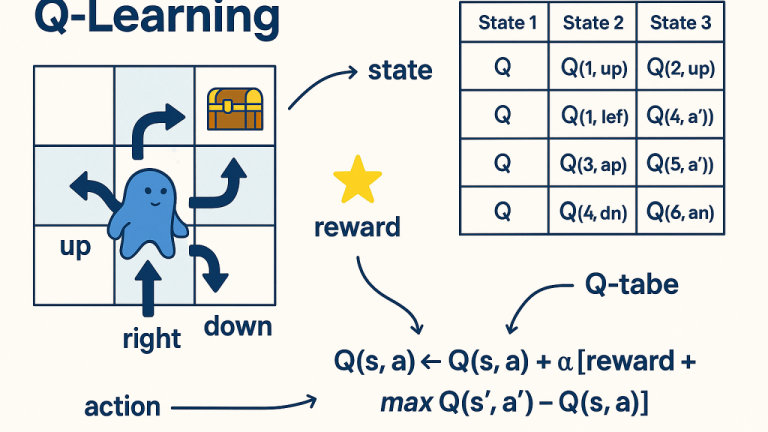
Reinforcement Learning (RL) is about learning through interaction. An agent takes actions in an environment, receives feedback as rewards (or penalties), and gradually improves its decisions to maximise long-term reward. Among the most widely taught RL methods is Q-learning, a simple but powerful algorithm that does not need a pre-built model of the environment. For learners exploring RL through a data scientist course in Chennai, Q-learning is often the first algorithm that makes the “trial, error, and improvement” idea feel concrete.
Q-learning is called model-free because it does not require transition probabilities or a simulator that predicts what will happen next. Instead, it learns directly from experience by estimating the value of taking a specific action in a specific state. Over time, those estimates guide the agent toward better behaviour.
What Q-Learning Actually Learns
At the heart of Q-learning is the Q-value, written as Q(s, a). It represents the expected future reward if the agent is in state s, takes action a, and then continues acting optimally.
Think of it like a scoreboard for decisions:
- State (s): where you are right now (e.g., a robot’s location).
- Action (a): what you can do (e.g., move left or right).
- Q(s, a): how good it is to take that action from that state.
Q-learning learns these values using the Bellman optimality idea: the best long-term decision now depends on the immediate reward plus the best possible value from the next state.
The Update Rule (The Engine of Learning)
Every time the agent takes an action and observes what happens, it updates its Q-value estimate. The classic Q-learning update is:
Q(s, a) ← Q(s, a) + α [ r + γ maxₐ’ Q(s’, a’) − Q(s, a) ]
Here’s what each term means:
- α (alpha): learning rate — how much you trust new information versus old estimates.
- r: immediate reward received after taking action a in state s.
- γ (gamma): discount factor — how much future rewards matter compared to immediate ones.
- s’: the next state reached.
- maxₐ’ Q(s’, a’): the best predicted value from the next state.
The bracketed part is called the temporal difference (TD) error: it measures how surprising the outcome was compared to what the agent expected. If the outcome is better than expected, Q increases; if worse, Q decreases.
Step-by-Step: How the Algorithm Works
A typical Q-learning loop looks like this:
- Initialise Q-values
- Start with Q(s, a) = 0 (or small random values) for all state–action pairs.
- Choose an action (exploration vs exploitation)
- Use a strategy like epsilon-greedy:
- With probability ε, pick a random action (explore).
- Otherwise, pick the action with the highest Q-value (exploit).
- Take the action and observe (r, s’)
- The environment returns a reward and the next state.
- Update Q(s, a)
- Apply the update rule using the observed reward and estimated future value.
- Repeat for many episodes
- Over enough interactions, the Q-table (or Q-function) improves.
This loop is simple enough to implement quickly, yet it captures the core learning dynamic used in more advanced RL systems.
Key Concepts That Determine Performance
Exploration vs Exploitation
If the agent always chooses what currently looks best, it may miss better options it has not tried yet. Exploration is essential early on. Many practitioners reduce ε gradually over time so the agent explores initially, then exploits more later.
Learning Rate (α)
- Too high: learning becomes unstable and overreacts to noisy experiences.
- Too low: learning becomes slow and may stall before reaching a strong policy.
Discount Factor (γ)
- Higher γ (close to 1): prioritises long-term reward (useful in multi-step tasks).
- Lower γ: focuses more on immediate reward (useful if far future is uncertain).
These parameters are where theory meets practice, and they are frequently tuned in hands-on labs in a data scientist course in Chennai when learners test RL agents on grid worlds, simple games, or simulated control problems.
Practical Considerations and Modern Extensions
When Q-Learning Works Best
Classic Q-learning is most effective when:
- The state and action spaces are small enough to store in a table.
- The environment is reasonably stationary (rules don’t change constantly).
- You can run enough episodes to learn reliably.
Limitations
In real-world problems, states are often huge or continuous (e.g., images, sensor streams). A simple Q-table becomes impossible. That is why function approximation is used: instead of storing Q-values in a table, you learn a model that predicts Q(s, a).
This leads to Deep Q-Networks (DQN), where a neural network approximates Q-values. While DQN adds complexity, the core idea remains the same: learn action values from experience without requiring an environment model—an idea frequently introduced after foundational Q-learning in a data scientist course in Chennai.
Conclusion
Q-learning is a foundational model-free RL algorithm that learns the value of taking an action in a given state by repeatedly interacting with an environment and updating its expectations. Its strength lies in simplicity: it does not need transition probabilities, it improves from raw experience, and it offers a clear bridge from basic RL concepts to deeper methods like DQN. If you want a practical starting point for reinforcement learning, Q-learning provides the cleanest path from intuition to implementation—exactly the kind of concept that benefits from structured practice in a data scientist course in Chennai.
